Method: Brownain Motion

Brownian Motion (or Wiener Process) is a basic ingredient of a model in describing stochastic evolution. This article shows how to simulate the motion of a varible (or particle) in 1-dimension using python. You will discover some useful ways to visualize the analyze the difference between different Brownian Motion model. Once you understand the simulations, you can tweak the code to simulate the actual experimental conditions in your study.

Packages used in the simulation:

from scipy.stats import norm     # For generating random numbers
import matplotlib.pyplot as plt  # For ploting purpose
import numpy as np

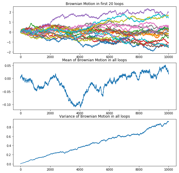
Model: Simple Brownian Motion

The code below shows how to stimulate the motion of a single particle in one-dimension. The motion is composed of a squence of normally distributed random displacement.

Given a fixed time increment $\Delta t > 0$. We consider

Hence, we divide the interval [0, T] into a grid such that

def BrownianMotion(N, T):
    
    # Step 0: Initial Condition
    dt = float(T)/N
    W = 0.
    W_all = [W]
    
    # Step 1: Draw random numbers Z from Gaussian distibution
    # Step 2: W <- W + sqrt(dt)*Z
    # Step 3: Repeat until i < N
    
    for i in range(1, N):
        W = W + np.sqrt(dt)*np.random.normal(loc = 0, scale = 1)
        W_all.append(W)
    return W_all

To calculate the deviation of motions in each timestep, we run the model for 100 times to acquire the following result:

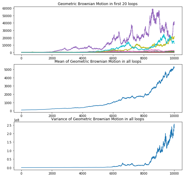
Model: Geometric Brownian Motion

For particles which only have non-negative moment (only move forward), Simple Brownian Motion is not approriate for modeling stock prices. Instead, a non-negative variation , named Geometric Brownian motion, takes care of the non-negativity feature.

def geoBrownianMotion(sigma, r, x, N, T):
    
    # Step 0: Initial Condition
    dt = float(T)/N
    S = x
    S_all = [S]
    
    # Step 1-4:
    for i in range(1, N):
        Z = np.random.normal(loc = 0, scale = np.sqrt(dt))
        S = S*np.exp((r - float(sigma**2)/2)*dt + sigma*(Z))
        S_all.append(S)
    return S_all

Same as the above, we run the model for 100 times to acquire follwing results:

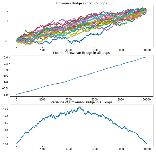
Model: Brownian Bridge

Brownian Bridge is a special model extend from Brownian Motion. The model allows controlling the position at specific time.

def BrownianBridge(x, y, N, T):
    
    # Step 0: Initial Condition
    dt = float(T)/N
    W = 0
    W_all = [W]
    t = 0
    t0 = 0
    # Step 1-4:
    for i in range(1, N):
        W = W + np.random.normal(loc = 0, scale = np.sqrt(dt))
        W_all.append(W)
    S_all = [x]
    for j in range(1, N):
        t = t + dt
        S_all.append(x + W_all[j] - \
                     (float(t- t0)/float(T - t0))* (W_all[-1]-y+x))
    return S_all

The result of Brownian Bridge has significant different features from the previous models: